
Velocity of Money: A Historical Market Perspective
Understanding how money flows through an economy provides crucial insights into market behavior, inflation patterns, and economic health. The velocity of money measures the frequency at which a unit of currency changes hands within a specific period, revealing much about consumer confidence, spending habits, and overall economic vitality. For those studying historical market movements, this metric offers a powerful lens through which to analyze past economic cycles, financial crises, and periods of expansion. By examining velocity trends across different eras, investors and researchers can identify patterns that inform contemporary decision-making and provide context for current market conditions.
The Foundation of Monetary Velocity
The velocity of money represents one of the most fundamental concepts in monetary economics, yet its implications extend far beyond theoretical frameworks. At its core, velocity measures how quickly money circulates through an economy, calculated by dividing nominal GDP by the money supply. When consumers and businesses transact frequently, velocity rises. When economic participants hold cash rather than spend it, velocity declines.
The quantity theory of money provides the mathematical framework for understanding this relationship. The famous equation MV = PQ states that the money supply (M) multiplied by velocity (V) equals the price level (P) multiplied by real output (Q). This elegant formula demonstrates how changes in velocity can affect price levels and economic output, assuming other variables remain constant.
Historical analysis reveals that velocity rarely stays constant. During the Roaring Twenties, rapid economic expansion and optimistic consumer sentiment drove velocity upward as money changed hands quickly through investments, purchases, and speculation. Conversely, the Great Depression saw velocity plummet as fearful households and businesses hoarded cash, creating a self-reinforcing economic contraction.
Measuring Velocity Across Time
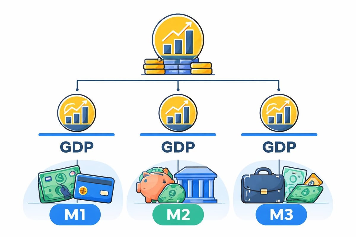
Financial historians employ several approaches to calculate the velocity of money, each offering unique insights into economic behavior. The most common measure divides GDP by M2, which includes currency, checking deposits, savings accounts, and money market securities. Alternative calculations use M1 (narrower) or M3 (broader) money supply definitions, producing different velocity readings.
Key measurement approaches include:
- GDP/M1 velocity: Captures transaction-focused money
- GDP/M2 velocity: Reflects broader money holdings
- Income velocity: Measures spending relative to income
- Transactions velocity: Accounts for all exchanges, not just final goods
Research exploring the determinants of velocity through life-cycle models expresses this metric as the reciprocal of the average holding time of money. This perspective emphasizes that velocity fundamentally measures how long people keep currency before spending it, providing a more intuitive understanding of the concept.
The digital age has introduced new complexity to velocity measurement. Cryptocurrencies and digital payment systems have prompted researchers to develop novel analytical frameworks. MicroVelocity analysis for digital currencies examines how wealth distribution affects circulation patterns, revealing heterogeneous behaviors that traditional aggregate measures might miss.
Historical Patterns and Crisis Periods
Examining velocity trends during major financial upheavals reveals consistent patterns that transcend specific historical contexts. The metric serves as a barometer of economic confidence, declining sharply during panics and recovering during expansions. These patterns offer valuable lessons for understanding market psychology and predicting potential turning points.
During the Panic of 1907, velocity contracted as banking uncertainties caused widespread hoarding. J.P. Morgan's intervention stabilized markets, but velocity remained suppressed for months as confidence slowly rebuilt. Similar dynamics appeared during the 1929 crash, when velocity's collapse amplified deflationary pressures despite Federal Reserve attempts to expand the money supply.
| Crisis Period | Velocity Trend | Primary Drivers | Recovery Timeline |
|---|---|---|---|
| Panic of 1907 | Sharp decline | Bank runs, uncertainty | 18-24 months |
| Great Depression | Sustained drop | Fear, deflation, unemployment | 8+ years |
| 1970s Stagflation | Volatile, elevated | Inflation expectations, instability | Variable |
| 2008 Financial Crisis | Historic plunge | Credit freeze, deleveraging | 6+ years |
| 2020 Pandemic | Rapid decline | Lockdowns, precautionary saving | Ongoing |
Analysis of velocity during financial crises from the Great Depression through the Great Recession demonstrates how financial innovation and regulatory changes affect circulation patterns. Each crisis presents unique characteristics, yet the fundamental relationship between uncertainty and velocity decline remains remarkably consistent.
The 2008 financial crisis provides particularly instructive lessons. Despite aggressive monetary expansion through quantitative easing, velocity continued falling as banks rebuilt capital and consumers deleveraged. This disconnect between money supply growth and economic activity challenged conventional monetary policy assumptions and highlighted velocity's critical role in transmission mechanisms.
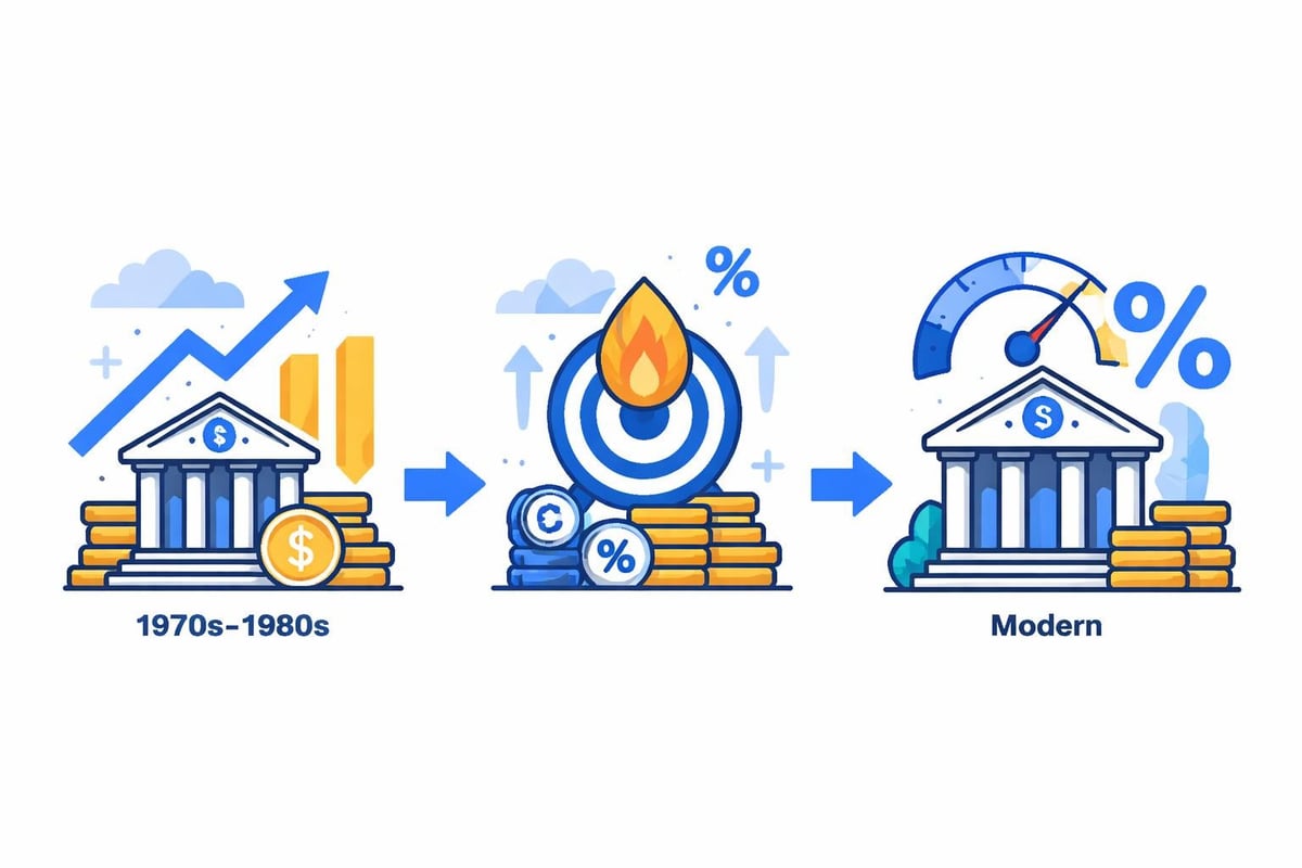
The 1970s Inflation Era
The stagflation period of the 1970s offers a contrasting case study where elevated velocity contributed to persistent inflation despite sluggish economic growth. Unlike depression scenarios where velocity collapses, this era saw money circulating rapidly as individuals sought to spend currency before inflation eroded its value. Understanding cash flow patterns during this period reveals how businesses adapted to changing monetary conditions.
Inflation expectations became self-fulfilling as rising velocity fed price increases, which in turn motivated faster spending. The Federal Reserve's eventual commitment to breaking this cycle through high interest rates succeeded partly by reducing velocity as the cost of holding money decreased and transaction demand fell.
Characteristics of 1970s velocity dynamics:
- Elevated velocity driven by inflation psychology
- Inverse relationship with interest rate policies
- Commodity hoarding as money substitute behavior
- International currency flows affecting domestic velocity
- Structural shift in financial instrument preferences
Velocity and Investment Strategy
For market participants analyzing historical patterns, velocity trends provide valuable context for understanding asset price movements and economic transitions. Rising velocity typically correlates with economic expansion, supporting equity valuations and business investment. Declining velocity often signals economic headwinds that may favor defensive positioning or fixed-income assets.
The relationship between velocity and asset prices isn't mechanical, but historical analysis reveals meaningful connections. During periods of accelerating velocity in the 1920s and 1950s, stock markets generally performed well as economic activity expanded. Conversely, velocity declines in 1930-1933 and 2008-2010 coincided with severe bear markets.
Bond markets demonstrate particular sensitivity to velocity changes through their impact on inflation expectations. When velocity rises rapidly, bondholders face increasing inflation risk, typically demanding higher yields. The interest coverage ratio becomes especially important for corporate debt analysis during these periods, as companies must service obligations while facing input cost pressures.

Regional and Sectoral Variations
Sophisticated historical analysis recognizes that velocity doesn't move uniformly across all economic sectors or geographic regions. Manufacturing-intensive economies may experience different velocity patterns than service-oriented ones. Urban areas typically demonstrate higher velocity than rural regions due to denser commercial activity and faster transaction frequencies.
During the post-World War II era, regional velocity differences within the United States reflected varying industrialization levels and population densities. Understanding these patterns helps explain why certain markets outperformed during specific periods and how capital expenditure cycles influenced local economic conditions.
Theoretical Frameworks and Models
Economic theorists have developed sophisticated models to explain velocity fluctuations and predict future trends. The comprehensive overview of velocity encompasses multiple theoretical perspectives, from classical quantity theory to modern behavioral approaches. Each framework offers insights relevant to historical market analysis.
The Cambridge cash balance approach emphasizes money demand rather than supply, framing velocity as the inverse of desired money holdings. This perspective helps explain why velocity changes during confidence shifts-when uncertainty rises, people increase desired cash balances, automatically reducing velocity.
More recent work on log-ergodic processes for modeling velocity offers new tools for analyzing long-term trends and understanding how velocity evolves over extended periods. These mathematical approaches help identify structural breaks in velocity patterns that may signal fundamental economic regime changes.
Major theoretical frameworks include:
- Classical quantity theory emphasizing mechanical relationships
- Keynesian liquidity preference focusing on interest rates and uncertainty
- Friedman's restatement incorporating permanent income concepts
- New monetarist models exploring search and matching dynamics
- Behavioral finance perspectives on money holding psychology
The Kiyotaki-Wright model provides a search-theoretic foundation for understanding how money emerges and circulates in decentralized economies. While abstract, this framework illuminates why velocity might vary based on transaction friction, trading patterns, and the availability of alternative exchange media.
Contemporary Relevance and Digital Evolution
Modern financial markets present new challenges for velocity analysis. Digital payments, cryptocurrencies, and innovative financial instruments complicate traditional measurement approaches. Yet the fundamental concept remains relevant, perhaps more so given how quickly digital money can circulate compared to physical currency.
The transition from traditional exchange mechanisms to digital platforms has potentially increased maximum velocity while also enabling more precise measurement. Payment processors track every transaction, providing granular data unavailable in earlier eras when cash transactions left no record.
| Era | Payment Technology | Typical Velocity | Measurement Precision |
|---|---|---|---|
| Pre-1900 | Cash, checks | Moderate | Low (estimates only) |
| 1900-1970 | Cash, checks, early cards | Moderate-high | Medium (sampling) |
| 1970-2000 | Cards, electronic transfers | High | Medium-high (partial tracking) |
| 2000-2026 | Digital payments, mobile | Variable, potentially higher | High (comprehensive data) |
Understanding historical money supply dynamics provides essential context for interpreting contemporary velocity trends. Central banks now navigate an environment where money can move globally in seconds, yet paradoxically, velocity in developed economies has trended downward since the 2008 crisis.
Policy Implications Through History
Monetary policymakers have long grappled with velocity's instability, which complicates efforts to control inflation and stabilize output through money supply adjustments. If velocity changes unpredictably, targeting money supply growth becomes less effective. This challenge has led central banks toward interest rate targeting rather than monetary aggregate control.
Historical episodes demonstrate both successes and failures in managing velocity through policy. The Volcker-era Federal Reserve successfully reduced velocity alongside inflation in the early 1980s through credible commitment to price stability. Conversely, attempts to stimulate velocity through monetary expansion during the Great Depression proved largely ineffective as liquidity preference overwhelmed supply increases.
The work of economists like David I. Meiselman on velocity stability helped shape monetary policy debates in the mid-20th century. His collaboration with Milton Friedman explored whether velocity followed predictable patterns that policymakers could exploit, ultimately concluding that while not constant, velocity exhibited some regularity in normal periods but could shift dramatically during crises.
Practical Applications for Market Analysis
Investors, researchers, and analysts can incorporate velocity analysis into their historical market studies through several practical approaches. Tracking velocity alongside price indices, output data, and financial market returns reveals relationships that single indicators miss. This multi-dimensional perspective strengthens pattern recognition and improves understanding of causal mechanisms.
When examining specific historical episodes, comparing velocity trends across different money supply measures provides insights into which types of money were driving circulation changes. For instance, if M1 velocity rises while M2 velocity remains stable, this suggests increased transaction activity without corresponding changes in broader money holding behavior.
Analytical techniques include:
- Plotting velocity against stock market indices to identify lead-lag relationships
- Comparing velocity trends across different countries during synchronized global events
- Analyzing velocity changes before and after major policy interventions
- Examining correlations between velocity and inflation across various time periods
- Studying velocity behavior during different phases of business cycles
The relationship between velocity and corporate spin-offs or other major restructuring events may seem indirect, but understanding broad economic context helps explain why certain corporate strategies succeeded or failed. During high-velocity periods with strong economic activity, restructurings often created shareholder value. During velocity collapses, even well-conceived strategies struggled amid broader economic malaise.
Learning From Velocity's Historical Lessons
Studying the velocity of money across different historical periods reinforces several enduring lessons. First, confidence matters enormously-velocity reflects not just mechanical transaction needs but also psychological willingness to engage in economic activity. Second, velocity can amplify both expansions and contractions, making it a crucial variable in understanding cycle dynamics. Third, structural changes in financial systems, payment technologies, and regulations can shift velocity patterns permanently.
The early contributions of economists like William Petty to understanding money circulation laid groundwork for modern velocity analysis. While his 17th-century observations lacked today's mathematical sophistication, his focus on how money moved through the economy rather than simply its quantity demonstrated remarkable insight into what would become a central concept in monetary theory.
For contemporary market observers, historical velocity analysis offers perspective on current debates about monetary policy effectiveness, inflation risks, and economic recovery prospects. When central banks expanded balance sheets dramatically after 2008 and again in 2020 without triggering runaway inflation, velocity's collapse explained much of this puzzle. Money creation doesn't automatically translate to spending or price increases if circulation slows commensurately.
The velocity of money provides a powerful analytical framework for understanding economic history and market behavior across different eras. By measuring how actively money circulates, this metric reveals crucial insights about consumer confidence, business activity, and the effectiveness of monetary policy interventions. Whether examining the Great Depression's deflationary spiral, the 1970s inflation surge, or modern post-crisis dynamics, velocity patterns help explain why markets behaved as they did and what lessons remain relevant today. Historic Financial News empowers investors, students, and researchers to explore these patterns through interactive historical data, AI-powered analysis, and comprehensive market context, transforming complex economic concepts into actionable insights that illuminate the stories behind market movements and help identify opportunities in contemporary markets.